AdS/CFT Duality in the Extraction of the AC-Conductivity of a Semi-Metal

Abstract

The AdS/CFT duality has been one of the most celebrated areas of research in the field of string theory, and here we give a brief introduction to it and follow up by utilizing it in an example calculation as a demonstration. Most physical theories involving particle interactions in metals involve weak coupling. Our project uses a way to understand the properties of a system with a large density of charged particles in a limiting case where the interactions between the particles is strong, which, due to the AdS/CFT duality between quantum field theories and solutions of string theory, makes the system more mathematically tractable because the fields in the Anti-de Sitter become weakly interacting. We will call this system a quantum semi-metal. We then proceed to utilize Maxwell's equations to extract the twopoint current correlation function of this object and its AC-conductivity, using a probe D₅-brane.

Preface

This is the report to conclude a directed project as part of the requirements to completing the PHYS 349 course at UBC. We present no original work, and this report is mostly a retelling of the story of the AdS/CFT duality from a combination of sources, mostly from the book "Gauge/Gravity Duality" by Martin Ammon and Johanna Erdmenger, "Introduction to the AdS/CFT Correspondence" by Jan de Boer [6], "The AdS/CFT Correspondence" by Veronika E. Hubeny [11] and "AdS/CFT Correspondence in Condensed Matter" by A.S.T Pires [15]. The calculations were directed by Dr. Gordon Walter Semenoff (Department of Physics, The University of British Columbia)

Table of Contents

Table of Contents.......................................................................................... iv

List of Figures................................................................................................ vi

Acknowledgments........................................................................................ vii

1 Introduction................................................................................................ 1

2 Taking the Large N Limit and Holography...................................................... 3

3 Anti-de Sitter Space..................................................................................... 5

4 Correlation Functions.................................................................................. 7

5 Derivation of the Ads/CFT Correspondence.................................................. 9

5.0.1 Mapping between parameters............................................................. 11

5.0.2 Turning off Quantum Fluctuations, and the weak form ofthe Correspondence 12

6 Probing a Strongly Correlated CFT with a D5-Brane..................................... 13

6.0.1 Maxwell's Action on the D5 Brane........................................................ 16

6.0.2 Extracting the AC-Conductivity............................................................. 21

7 Epilogue.................................................................................................... 25

Bibliography................................................................................................ 27

List of Figures

Figure 6.1 A D5 brane is held perpendicular to a stack of an infinite number of coincident D3 branes that are at r = 0. The stack of D3 branes extends along the spacetime directions x⁰,x¹,x²,x³, and are transversal to the other six spatial directions x⁴,...x⁹ . In the limit depicted in the figure, the strings in the bulk are rigid, and we solve Maxwell's equations on the surface of the D5-brane to extract the two-point current correlation function at the boundary (r = ∞). In essence, we are looking for this particular operator on the "upper edge" of the infinite square depicted as the D5 brane in this figure. . . . . . . . . . . . . . 14

Introduction

The AdS/CFT Correspondence has become very important in the last two decades, with thousands of papers having been published in high energy Physics. While still a conjecture not having been proved, there is substantial evidence to believe that it holds. One reason for its importance is that it can be used to understand strongly interacting field theories by mapping them into classical gravity in one extra dimension. The idea is that large-N gauge theories (strongly coupled conformal field theories) in d-dimensions is mapped to a gravitational theory in d+1 dimensions which is asymptotically AdS. This happens to be a strong-weak duality where if for example, the field theory is strongly coupled, the gravity theory is weakly coupled and vice versa. The most well-known form of this that the correspondence takes, originally conjectured by Maldacena [12], is that between 4-dimensional N = 4 supersymmetric Yang-Mills theory and type IIB string theory on AdS₅ ×S⁵ - which is a 10-dimensional world where AdS₅ refers to Anti de-Sitter space in 5 dimensions and the S⁵ to a 5-dimensional sphere. Anti-de Sitter spaces are maximally symmetric solutions of the Einstein equations with a negative cosmological constant [6]. N = 4 super Yang-Mills theory was known to be conformally invariant (making this quantum field theory a conformal field theory, or a CFT), and it turns out that its group of conformal symmetries matches up exactly with the large symmetry group of 5-dimensional Anti-de Sitter space. Different CFTs in d-dimensions will generally correspond to theories of gravity with different field content and different parameters in the bulk (d+1 dimensions). Different arguments have shown that quantum field theories are actually quantum theories of gravity and so we can use them to compute observables of the QFT when the gravity theory is classical [13]. This fact we will use in this report.

Notice that the AdS/CFT correspondence takes a gravity theory in d+1 dimensions and relates it to a non-gravitational one in d-dimensions. String theory provides a means to compute finite quantum corrections to classical gravity, but its full non-perturbative structure is still not well understood [6]. If the AdS/CFT correspondence is true, this means that the actual quantum degrees of freedom cannot be the same as that of a local field theory that lives on the same space. If gravity had degrees of freedom that were local, we could take arbitrarily large volumes of fixed energy density - but we know from classical gravity that such a thing would eventually collapse to form a black hole. Clues for this gauge-gravity duality have been around for some time - in three dimensions in particular . It turns out that in the 3dimensional case, gravity can be described by Chern-Simons theory [1, 22].ChernSimons theory is a topological field theory that reduces to a 2-dimensional field theory when put in a manifold with a boundary [21] [6]. A precise relation between Hilbert spaces and correlation functions in compact gauge groups could be established - while for non-compact gauge groups this precise relationship is not well understood. Nevertheless this duality between Chern-Simmons theory and two-dimensional conformal field theory has many similarities to the AdS/CFT duality [6].

Here we will primarily work with a weaker form of the AdS/CFT correspondence by working in the low-energy limit in the string theory side. At very low energies, it is known that type IIB string theory on AdS₅ ×S⁵ reduces to type IIB supergravity on AdS₅ ×S⁵. Correspondingly, we end up taking a limit on the N = 4 supersymmetric field theory side where the rank of the U(N) gauge group, N (not the same as the earlier N) and g_YM² both become large. In this limit, the equivalence between type IIB supergravity on AdS₅ ×S⁵ and N = 4 gauge theory has been well tested [6].

Taking the Large N Limit and Holography

The AdS/CFT correspondence is associated to two ideas in Physics. The first is that large N gauge theory is equivalent to a string theory [19]. In terms of 1/N and g_YM² , the perturbative expansion of a large N gauge theory has the following form:

Z = ∑ N^2−2g f_g(λ) (2.1)

g≥0

where λ = g_YM² N is called the 't Hooft coupling constant. This is reminiscent of the loop expansion in string theory:

Z Z_g (2.2)

g≥0

- if we replace the string coupling constant g_s with 1/N. Through some mechanism, Feynman diagrams of the gauge theory are turned into surfaces that represent strings [14] - and apparently this is exactly what happens in the AdS/CFT correspondence.

The second idea in Physics is that of "holography" [17, 20]. This idea is related to the thermodynamics of black holes. Hawking and Bekenstein showed that black holes can be seen as thermodynamic entities [4, 5, 9].Thus they have entropies and temperatures. The black body radiation that the black hole emits relate directly to its temperature, while its entropy is given by S = c³A/4Gh¯, where A is the surface area of the event horizon of the black hole, and G the Newton constant. These definitions make the laws of thermodynamics consistent with Einstein's equations of general relativity. The entropy of a system can be viewed as its "information content". It is a measure of the number of degrees of freedom that a theory has - and so it is surprising that the entropy of a black hole scales with its horizon area, and not its volume. Local field theories have their entropies proportional to their volume, so it cannot be that gravity behaves like a local field theory. It turns out that if we assume that gravity in d +1 dimensions is somehow equivalent to a local field theory in d dimensions, we reach a consistent picture. This is where this idea in Physics gets its name of "holography"- it is like a hologram where 3-dimensional information is encoded in a 2-dimensional surface. The AdS/CFT correspondence is therefore holographic, since it states that quantum gravity in 5dimensions (forgetting the 5-sphere) is equivalent to a field theory in 4 dimensions [6].

Anti-de Sitter Space

The Anti-de Sitter space belongs to a wide class of homogeneous spaces that can be defined as quadric surfaces in flat vector spaces [15]. An example is the ddimensional sphere S^d given by:

X (3.1)

embedded in Euclidean d+1 dimensional space. The d-dimensional anti-de Sitter space can be defined:

d−1

X R² (3.2)

i=1

embedded in flat d+1 dimensional space with the metric:

d−1

dsdX_i² (3.3)

i=1

This has constant negative curvature [15].Of course, this can be written in different coordinate systems, and in the Poincare coordinates´ (r,t,~x),r > 0,~x ∈ R^d−2 given by [2]:

X₀ = 1 [1+r²(R² +~x² −t²)], X_d = Rrt

2r

Xⁱ = Rrxⁱ, (i = 1,....,d −2)

Xd−1 = [1−r2(R2 −~x2 +t2)], 2r the anti-de Sitter metric then becomes

(3.4)

¹

ds (3.5)

grr ,

gxx = gyy = gzz = r2,

gtt = −r2

(3.6)

r

The limit where the radial coordinate r goes to infinity is called the boundary of the anti-de Sitter space . The boundary is the place where the dual field theory lives [6]. It turns out that string theory excitations extend all the way to the boundary of the space [7]. In this way it is possible to obtain a map from string theory states in the bulk to states in the field theory living in the boundary. It also seems that r can be seen as a dimension of scale of the dual field theory [18].

Correlation Functions

Maldacena's paper [12], proposed a form of the AdS/CFT correspondence but did not yet provide a map between the two sides. In [23] and [8] such a map was given and makes the correspondence clear. To illustrate, we consider a free field with a mass m on the AdS side, propagating in anti-de Sitter space. We see that the field equation:

(+m2)φ = 0 has two linearly independent solutions that behave like [6] :	(4.1)
e−∆r, e(∆−4)r as r → ∞, where	(4.2)
∆(∆−4) = m2	(4.3)

Now let us consider a solution of the supergravity equations of motion , possessing the boundary condition that near r = ∞ , the fields behave as [6]:

e(∆−4)r (4.4)

The map between AdS and CFT quantities is then given by:

exp −S_sugrav (4.5)

The left hand side of the above is the supergravity action evaluated on the classical solution given by φ_i , with the right hand side being a generating function for correlation functions in Yang-Mills theory [6]. For most applications, the above suffices, but it's important to note that the left hand side is really an approximation - and we should really use the full string theory partition function subject to the relevant boundary conditions, to which our supergravity approximation is a saddlepoint approximation [11]:

Z_string (4.6)

We see that there is an operator O_i in Yang-Mills theory corresponding to every bulk field φ_i (in AdS). We can use symmetries to find which boundary operators (in the field theory side) , map to which fields (in the bulk, that is, the AdS side). The two sides must have the same quantum numbers and Lorentz structure [11].As an example, conserved currents in the field theory side correspond to global symmetries and therefore their corresponding sources act as external background gauge fields, which are boundary values of dynamical gauge fields in the AdS side (the bulk) [11]. We will use the above to find the "two point" current correlation function in the subsequent sections.

Derivation of the Ads/CFT Correspondence

To do the derivation of the AdS/CFT correspondence given in Maldacena's original paper [12], we need the idea of D-branes (or Dirichlet branes). Polchinski introduced them in [16] as extended objects in string theory. The number of spatial dimensions they have give them a label - D0 branes are like particles, D1 branes are strings , D2 branes are like sheets etc. We have two ways to think about D-branes . The first one is as solitonic solutions to the equations of motion of low energy string theory , that is, of supergravity . (this perspective is reliable for g_sN >> 1 , to be explained shortly) - known as the "closed string perspective" [3], the D-branes act as sources of a gravitational field which curves the surrounding spacetime, and the characteristic length "R" (we will explain this shortly) is large to ensure the validity of the supergravity approximation [3] and the second way to think about D-branes is as higher dimensional objects where open strings can end. Open strings have finite tension, and their center of mass cannot be taken arbitrarily far away from a D-brane [6]. Consequently, the degrees of freedom of the open string are confined to in a direction parallel to the D brane. It's important to note that both the open and closed string perspectives have their advantages, and as we shall see, with a stack of D3 branes, and taking a certain limit the open string description reduces to N = 4 super Yang-Mills theory while the closed string perspective reduces to string theory on AdS₅ ×S⁵ - thus the AdS/CFT correspondence arises as a consequence of the duality between open and closed strings.

Let us consider N coincident D3 branes (these have three spatial dimensions and a time dimension) in type IIB string theory. g_s is the string coupling constant, which governs the strength of the interactions between open and closed strings. The coupling constant is g_sN. At weak coupling g_sN << 1 the branes live in ta 10-dimensional flat spacetime with open strings ending on the D branes and closed strings in the bulk. At strong coupling g_sN >> 1 the spacetime is substantially curved by the branes, sourcing the extremal black 3-brane geometry [10]:

ds2 −1/2 µ ν + f(r)1/2(dr2 +r2dΩ25), f(r) = 1+ 4πgs4Nls4 (5.1) = f(r) ηµνdx dx

r

where dΩ²₅ is the metric of a unit 5-sphere (S⁵), l_s is the string length and x^µ

denotes the 4 coordinates along the D3 brane world volume. The solution has a self-dual 5-form field strength which has a flux on the S⁵ here [11].

We have seen two regimes of g_sN : g_sN << 1 and g_sN >> 1, with apparently no overlap. The insight that Maldacena had was to decouple the theory on the branes from gravity - which can be done by taking a low energy limit that simplifies things a lot. The open string sector decouples from the rest of the theory and we end up with an SU(N) Yang-Mills theory that describes the dynamics of the branes. On the other hand, this limit in the black-brane spacetime in the near horizon geometry - asymptotically, any near-horizon finite energy excitation is strongly redshifted, while modes that propagate in the asymptotic region of 5.1 decouple from the region near the horizon since its cross section vanishes in this limit [11].

The event horizon r = 0 of the black brane solution 5.1 lies at infinite proper distance from spacelike geodesics - so its embedding diagram has an infinite "throat". The near horizon geometry then simplifies to a product of a sphere and Antide-Sitter spacetime [11].The near-horizon geometry here is this 10-dimensional AdS₅ ×S⁵.

Now in 5.1, if we define R = (4πg_sN)^1/4l_s, we note that as r → 0, that is as we

zoom in on the horizon, f(r) → R²/r², and we end up getting:

² r2 R2 2 2 2

ds = R² η_µνdx_µdx_ν ⁺ r₂ dr +R dΩ5 (5.2)

The first two terms above describe AdS₅ (something which we've seen before)a maximally symmetric spacetime of constant negative curvature, with a radius of curvature of R, while the last term describes the sphere S⁵ (also with radius R). The D-branes are not localized in the geometry anymore, but their effect is manifested in the 5-form flux through the sphere S⁵ [11].

Our stack of D3-branes in the low energy limit is then described by a 10dimensional string theory with closed strings when g_sN >> 1 in AdS₅ ×S⁵, and by 4-dimensional super Yang-Mills SU(N) field theory when g_sN << 1. But the gauge theory is defined at any value of the coupling constant, and so we can conjecture that it holds even when g_sN is large - the same regime where the closed string description holds [11]. It was this observation that led Maldacena [12] to conjecture:

(String theory on AdS₅ ×S⁵) = (N = 5, SU(N) gauge theory in 4D)

In other words, the two sides describe the same physics - it's a full duality.

5.0.1 Mapping between parameters

The AdS/CFT duality is an example of a weak-strong coupling duality. The correspondence specifies how the parameters on the two sides - the field theory side and the bulk, relate to each other. On AdS₅ ×S⁵, string theory has a dimensionless coupling constant g_s , which determines the strength of the interactions between strings splitting and joining, and the string length l_s that sets the size of the fluctuations of the string world sheet,, and another parameter R which as we've seen before, is the radius of curvature of AdS₅ ×S⁵.

4-dimensional N = 4 super Yang-Mills theory with gauge group U(N) has of course, the rank N of the gauge group and a dimensionless coupling constant that we've seen before - g_YM² . The parameters between the two sides relate to each other in the following way [6]:

, (R/l_s)⁴ = 4πg_YM² N = 4πλ (5.3)

λ in the above equation is the 't Hoooft coupling constant.

5.0.2 Turning off Quantum Fluctuations, and the weak form of the Correspondence

For our purposes, we turn off quantum fluctuations and suppress any stringy corrections of the geometry, so we take g_s << 1, while keeping R/l_s constant. To leading order in g_s then, the AdS side reduces to classical string theory. The string length l_s (which is measured in units of R)is kept constant. This we refer to as the strong form of the AdS/CFT correspondence [3]. Looking at 5.3 we see that on the CFT side this implies taking g_YM << 1 while g_YM² N stays finite. This means that we have to take the large N limit, N → ∞ for a fixed λ, which is called the 't Hooft limit. In this limit, there is only one free parameter on each side - on the CFT side we have λ, and on the string theory side, we have the radius of curvature R/l_s (remembering we kept l_s constant). Then 5.3 tells us that these two parameters are related by (R/l_s) = λ^1/4. We want to work with a strongly correlated material, so we take the limit λ → ∞ - that is, the material (on the CFT side ) is infinitely coupled - and we see that on the string theory side this corresponds to the limit R → ∞. The string length is then very small compared to the radius of curvature, and we see that we have obtained the point-particle limit of type IIB string theory, which is given by type IIB supergravity on AdS₅ ×S⁵. Thus we have a strong-weak duality - strongly coupled N = 4 Super Yang-Mills is mapped to type IIB supergravity on weakly curved AdS₅ ×S⁵ space. This special limit is known as the weak form of the AdS/CFT conjecture [3]. We see that due to this duality, we can solve for strongly coupled systems on the CFT side much more easily on the gravity side the mathematics becomes tractable.

Probing a Strongly Correlated CFT with a D5-Brane

The AdS/CFT duality tells us that every bulk field φ corresponds to an operator O in the gauge theory. Now we want to take a strongly correlated material (for which we assume λ = ∞, given by a CFT, and wish to extract its AC-conductivity. Because of the coupling constant λ showing up in perturbative expansions, they diverge and the mathematics is thus not tractable. However, in chapter 5 we have seen that there is a dual problem we can solve on the AdS side, which, for this value of λ, would be a problem on a weakly curved spacetime with no stringy interactions. We wish to find the two-point current correlation function for this strongly correlated object, which we will call a semi-metal, and its AC-conductivity.

We use the weak form of the AdS/CFT duality as talked about in chapter 5, and we set up a "probe" D5-brane perpendicular to our stack of infinite number of coincident D3 branes at r = 0 (Figure 6.1).

We will solve Maxwell's equations on the surface of this D5-brane, and so we will suppress one spatial direction (without loss of generality, let this suppressed direction be the z-direction). The geometry of this surface is thus AdS₄ ×S². The two point current-current correlation function at r = ∞ , < j^µ(x)j^ν(y) >, where j^µ and j^ν are current-density operators, defined at two points x and y. This implies we need infinite resolution, and as pointed out in chapter 6, since the r dimension is a dimension of scale, this corresponds to our operators living at r = ∞.

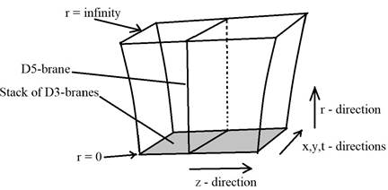
Figure 6.1: A D5 brane is held perpendicular to a stack of an infinite number of coincident D3 branes that are at r =0. The stack of D3 branes extends along the spacetime directions x⁰,x¹,x²,x³, and are transversal to the other six spatial directions x⁴,...x⁹ . In the limit depicted in the figure, the strings in the bulk are rigid, and we solve Maxwell's equations on the surface of the D5-brane to extract the two-point current correlation function at the boundary (r = ∞). In essence, we are looking for this particular operator on the "upper edge" of the infinite square depicted as the D5 brane in this figure.

We recall that Maxwell's equations in Lorentz covariant form are:

∂µFµν = jν, Fµν = ∂µAν −∂νAµ (6.1)

And an equivalent form of Maxwell's equations in a curved spacetime is:

µρ

g(6.2)

We have the fields A_b(r,x,y,t) on the surface of the D5 brane (the bulk field), and we set the boundary conditions:

lim A_b(r,x,y,t) → a_b(r), lim A_b(r,~x) = 0 (6.3) r→∞ x,y,z→∞

It is known from chapter 4, that we can put a_b(r) into equation 4.5 to get correlation functions, which in this case will turn out to be the current-current correlation functions.

< ei^R a_µ j^µ >= e−S[a] (6.4)

where we use the Born-Infeld Action, S, from string theory on the right hand side.

The left hand side is expanded as:

< e dx₁...dx_n a_µ

n=0 n!

< eiR aµ jµ

(6.5)

while we expand the right hand side of equation 6.4 as:

^{R µ} Z

e−S[a] = < ei a_µ j > = 1−n aρ∆a_ρ +.. (6.6)

where ∆ in the equation above is some operator to be identified. Putting 6.5

and 6.6 together we get:

Comparing 6.6 and 6.7, we see that the operator ∆ is in fact the two-point current correlator < j^µ(x)j^ν(y)> , the operator that we seek, and whose coefficient will tell us the AC-conductivity of our strongly correlated material. We see that ∆ is obtained from the quadratic term in 6.6. In the low energy limit (the regime we are working in here) , the Born-Infeld action can be approximated by the Maxwell action, and it turns out that this approximation for S at the boundary, evaluated with the boundary conditions 6.3, give us the quadratic term when we insert it into 6.6. We will first show this and get the current-current correlation function in the next section, and then fix its coefficient (the AC-conductivity) in the section that comes after that.

6.0.1 Maxwell's Action on the D5 Brane

Given the D5 brane metric 3.6, we intend to solve 6.2 in the case where j^ν = 0 with the boundary conditions 6.3. So we want to solve:

pµρ νσ = 0

∂µ −detg g g Fρσ

⇒ ∂_µ^p−detg g^µµg^ννF_ρσ = 0 (6.8)

For this section, we will ignore the parameter R in the metric, for reasons that will be made clear in the next section, 6.0.2. Choosing ν = r, let µ = a = x,y,t (this "a" has nothing to do with our boundary condition, it is just an index here).

Putting into 6.8:

∂a(r2r2gaaFar) = 0 r4∂a(gaaFar) = 0

r²∂_a(∂^aA^r −∂^rA^a) = 0 (6.9)

Using our freedom to choose a gauge, we choose one such that A_r = A^r = 0.

Thus, 6.9 becomes:

r2∂r[∂a(Aa)] = 0 For ν = x,y,t, we have:

(6.10)

p^{µµ bb} = 0

∂_µ −detgg g F_µb

∂a −detggaagbbFab +∂rp−detggrrgbbFrb = 0 p (1/r2)∂a(Fab)+∂r(r2Frb) = 0 (1/r2)∂a(∂aAb −∂bAa)+∂r(r2∂rAb −r2∂bAr) = 0
(1/r2)∂a(∂aAb −∂bAa)+∂r(r2∂rAb) = 0 We multiply 6.11 by r2,	(6.11)
∂a(∂aAb −∂bAa)+r2∂r(r2∂rAb) = 0	(6.12)

Using gauge invariance, we choose ∂_aA^a = 0 (and it follows from 6.10 that ∂_aA^a = 0 at r = 0 as well - it has no r dependence) So for a 6= b, 6.12 is:

∂a(∂aAb)+(r2∂r)(r2∂r)(Ab) = 0 Using separation of variables, we set the following condition:	(6.13)
Ab(r,~x) = Ab(r,k)eikcxc	(6.14)

where^~k is a vector in momentum space having modulus k. Putting this into 6.13:

−k_ak^aA_b +(r²∂_r)(r²∂_r)(A^b) = 0

∂ −k2A_b = 0 (6.15)

A_b

We set Aa(r,k) at r = 0 to be finite and:
lim Aa(r,k) = aa(k) r→∞ Now let (1/r) = σ, so 6.15 becomes:	(6.16)

0 (6.17)

The above equation has the general solution:
Ab =C1ekσ +C2e−kσ	(6.18)

The fact that we set A_b to be finite at r = 0 gives us C₁ = 0 in 6.18, and

6.16 implies C₂ = a_b(k). So we get the solution:

Ab(σ(r),k) = ab(k)e−kσ = ab(k)e(−k/r) Putting the above into 6.14, we obtain:	(6.19)
Ab(r,~x) = eikcxcab(k)e−k/r	(6.20)

Since 6.17 is a homogeneous equation, a superposition of solutions is still a solution. So we take a superposition of solutions of the form 6.20 :

^{Z c} −k/r 3

A_b(r,~x) = eikcx a_b(k)e d k

^{Z ikcxc}−k/ra_b(k)d3k (6.21)

= e

We are now in a position to plug the solution 6.21 into the Maxwell action, given by:

Z

drdgµνgρσFµρFνσ

Z

= drdg^µνg

Z

= drdgµνg

Z

= drdgµνgρσAgµνg

(6.22)

The second term in 6.22 is just 0, because it is a solution to Maxwell's equations. So 6.22 turns to:

Z

drdgµνg

Z

= drdgµµgρσA_ρF_µσ] (6.23)

We take r → ∞, and use Stokes' Law on 6.23 to obtain:

grrg

grrg (6.24)

Since A_r = 0, ∂_σA_r = 0 in 6.24. Continuing:

grrg

grrg

(6.25)

The above is what the Maxwell action has been reduced to at r → ∞. Finally, we plug 6.21 into 6.25:

#

eikcx^c eimcx^c−(m/r)a_ρ(m)d3m

eik_cx^c−(k/r)aρ(k)d3k^Z eim_cx^c

" #

Z

= me−k/raρ(k)e−m/raρ(m)d3k d3m ∂3(k+m)

m

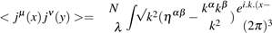
where in the last step, we have relabeled m = k for convenience. As promised before, the Maxwell's action does indeed give the quadratic term in 6.6 from which to extract ∆ , which we identified as the current-current correlation function by comparing with 6.7. We note that in our case, we assume that there is no net outflow or inflow of charge, so the conservation of charge tells us ∂_µ j_µ = 0. Hence we must have ∂_µ < j^µ(x)j^ν(y) >= ∂_µ∆^µν = 0, which, when Fourier transformed, gives us k_µ∆^µν(k) = 0. So we need to figure out what operator fits into 6.26 and satisfies these conditions. We see that the following works:

√ k^αk^β

< jα(k)jβ(−k) > = k2(ηαβ − k2 ) To check that it satisfies the conditions just outlined above:

(6.27)

!

k_µ

k kµkν

= k_µηµν − µ

= k^ν −

k2

= 0 (6.28)

We also need to check if we can somehow get 6.27 from 6.26 by re-writing the expression in 6.26 (essentially just adding zero to the expression), that is - we need to make sure we have not "changed" the expression. We recall that since we have let the bulk field approach a_µ(x^µ) (the Fourier transform of a_µ(k)) as r → ∞, from 6.10 we see that we must have ∂_µa_µ = 0, whose Fourier transform is k^µa_µ = 0.

With this piece of information:

d³k

!

a_ν(k)d³k

ka^µ

k (6.29)

6.29 is exactly 6.26 , just with the up and down indices switched - the last line in 6.29 follows because k^µa_µ = 0, making the second term on the third line zero. Thus, 6.27 gives the two point current correlation function for our strongly correlated semi-metal (called a semi-metal because it does not have a Fermi surface like metals do - but a Fermi point). Now what remains is to fix its coefficient and thus extract the AC-conductivity.

6.0.2 Extracting the AC-Conductivity

We now show that our approximation of the Born-Infeld action as the Maxwell action was justified and then we fix the coefficient of 6.27.

The Dirac-Born-Infeld Action is:

d6σqdet(g+2πα0Fµν) (6.30)

where the coefficient in the above expression is the D5-brane tension,

and the D5 brane metric (corresponding to g) is:

ds (6.31)

where the other variables are the same as ones considered before, with the last two terms coming from the sphere S⁵.

6.30 can be re-written as:

q

d6σ det(g).det(¹+2πα0g−1F)

dTr ln (6.32)

The trace of a symmetric matrix times an anti-symmetric one is zero, so:

∑ g−µν1 Fνµ = 0 (6.33)

µν

6.32 then becomes:

2Trg−1F g−1F d

Tr g

Tr g⁻¹ F g⁻¹ F (6.34)

where the term taken in the expansion above leads to the quadratic term in 6.6 as we will see, because it can be shown that the expression is a manifestation of Maxwell's action, which in the last section has been shown to lead to the quadratic term. In 6.34 above, we get a factor of R⁶ from the determinant, and a factor of 1/R⁴ from the trace, which will add an overall factor of R² to 6.34. Furthermore, we can re-write the trace in 6.34 as:

Tr g−1 F g−1 F

µµ

µ

⁼ ∑ g−1 µν F_νρ g−1 ρσ F_σµ

µ

= gµµ gρσ FµρFνσ (6.35)

Putting 6.35 into 6.34 and taking out the R² factor to the front gives us:

Rp (g) gµνgρσF_µρF

dtdxdydr det

We see that the rightmost quadruple integral in the expression above is the Maxwell action. So we were justified in approximating the Born-Infeld action this way. We also note that the R² factor was taken out to the front in the expression above, so det(g) there is different from the det(g)'s that came before it in the sense that it does not contain any factors of R, and this is the reason we ignored the R factors of the metric in the last section 6.0.1. Continuing to work with 6.36 should therefore give us the coefficient of the current-current correlation function (the AC-conductivity of the semi-metal). We compute the integrals over θ and φ, giving us a factor of 4π, that we take out to the front:

dtdxdr^pdet(g) g^µνg^ρσF_µρF (6.37)

We recall that λ = g_YM² N and g_s = (4πN/λ)⁻¹, so we can re-write the coefficient outside the brackets in 6.37 as:

√

24π3 λα03 4πN

(6.38)

It turns out that if we evaluated the interactions at the boundary in the field theory, we would get a potential that goes like g_YM/(4π |~x |), where |~x | is the distance between the two interacting entities. This is like a Coulomb potential, so g_YM is like a "charge" on our boundary. Multiplying 6.38 by g_YM² , we obtain the AC-conductivity:

(6.39)

For weakly correlated materials with a low coupling constant λ, the AC-conductivity scales like λ, while for our calculation with the D5 brane, it appears that this con-

√

ductivity scales like λ. The slower rate of increase of the conductivity with λ for strongly correlated systems is evidence of some "screening" taking place.

Now that we have fixed the coefficient of the current-current correlation function, 6.27 becomes:

√ α(k)jβ(−k) > = 2 πλ√k2(ηαβ − kαkk2β ) < j

(6.40)

The above gives our current-current correlation function in momentum space, so we do an inverse Fourier transform on 6.40 to obtain what we present as our two-point current correlation function:

2√ y) d₃k (6.41)

π

Epilogue

Black holes were once seen as a problematic, potential flaw in general relativity in the first half of the twentieth century. But they have moved on from that status to being astrophysical objects that we now have evidence for, and have become fascinating mathematical objects. The study of black holy entropy has motivated the advances in string theory which provided its basic framework [11], and extremal black branes have supplied the context for the derivation of the AdS/CFT correspondence. This correspondence is profound in that it relates a non-gravitational theory to a gravitational one, and it turns out that large black holes in AdS encode the dynamics of fluids and describe a vast array of systems that can be probed experimentally [11]. The AdS/CFT correspondence was used in this report to make a mathematically intractable problem involving a strongly correlated system into a mathematically tractable one, which allowed us to extract the two point currentcurrent correlation function and the AC-conductivity for what we called a semimetal. The correspondence can also be used to study finite temperature real time processes, examples of which are response functions and dynamics far from equilibrium in quantum critical points in condensed matter systems [15]. Computing these problems are made much simpler using the correspondence - if the original theory has d dimensions, solving them is reduced to solving classical gravitational problems in d +1 dimensions. The AdS/CFT correspondence is not only a useful playground in solving these problems, but it is also weaved into the exploration of the connections between quantum information and gravity. The most fascinating part of the AdS/CFT correspondence it seems, is that it connects so many apparently disparate ideas together, and it is likely to be a key ingredient in the unraveling of quantum gravity.

Bibliography

[1] A. Achucarro and P. K. Townsend. A Chern-Simons Action for Three-Dimensional anti-De Sitter Supergravity Theories. Phys. Lett., B180: 89, 1986. doi:10.1016/0370-2693(86)90140-1. [,732(1987)]. → page 2

[2] O. Aharony, S. S. Gubser, J. Maldacena, H. Ooguri, and Y. Oz. Large N field theories, string theory and gravity. Physics Reports, 323:183–386, Jan. 2000. doi:10.1016/S0370-1573(99)00083-6. → page 5

[3] M. Ammon and J. Erdmenger. Gauge/Gravity Duality: Foundations and Applications. Cambridge University Press, 2015. doi:10.1017/CBO9780511846373. → pages 9, 12

[4] J. D. Bekenstein. Black holes and entropy. Phys. Rev. D, 7:2333–2346, Apr 1973. doi:10.1103/PhysRevD.7.2333. URL https://link.aps.org/doi/10.1103/PhysRevD.7.2333. → page 3

[5] J. D. Bekenstein. Generalized second law of thermodynamics in black-hole physics. Phys. Rev. D, 9:3292–3300, Jun 1974. doi:10.1103/PhysRevD.9.3292. URL https://link.aps.org/doi/10.1103/PhysRevD.9.3292. → page 3

[6] J. de Boer. Introduction to the ads/cft correspondence. 2003. → pages iii, 1, 2, 4, 6, 7, 8, 9, 11

[7] J. de Boer, H. Ooguri, H. Robins, and J. Tannenhauser. String theory on AdS₃. Journal of High Energy Physics, 12:026, Dec. 1998. doi:10.1088/1126-6708/1998/12/026. → page 6

[8] S. S. Gubser, I. R. Klebanov, and A. M. Polyakov. Gauge theory correlators from non-critical string theory. Physics Letters B, 428:105–114, May 1998. doi:10.1016/S0370-2693(98)00377-3. → page 7

[9] S. W. Hawking. Black holes and thermodynamics. Phys. Rev. D, 13: 191–197, Jan 1976. doi:10.1103/PhysRevD.13.191. URL https://link.aps.org/doi/10.1103/PhysRevD.13.191. → page 3

[10] G. T. Horowitz and A. Strominger. Black strings and P-branes. Nucl. Phys., B360:197–209, 1991. doi:10.1016/0550-3213(91)90440-9. → page 10

[11] V. E. Hubeny. The AdS/CFT correspondence. Classical and Quantum Gravity, 32(12):124010, June 2015. doi:10.1088/0264-9381/32/12/124010. → pages iii, 8, 10, 11, 25

[12] J. Maldacena. The Large-N Limit of Superconformal Field Theories and Supergravity. International Journal of Theoretical Physics, 38:1113–1133, 1999. doi:10.1023/A:1026654312961. → pages 1, 7, 9, 11

[13] J. McGreevy. Holographic duality with a view toward many-body physics. ArXiv e-prints, Sept. 2009. → page 2

[14] H. Ooguri and C. Vafa. Worldsheet derivation of a large /N duality. Nuclear Physics B, 641:3–34, Oct. 2002. doi:10.1016/S0550-3213(02)00620-X. → page 3

[15] A. T. Pires. Ads/CFT correspondence in condensed matter. ArXiv e-prints, June 2010. → pages iii, 5, 25

[16] J. Polchinski. Dirichlet Branes and Ramond-Ramond Charges. Physical Review Letters, 75:4724–4727, Dec. 1995. doi:10.1103/PhysRevLett.75.4724. → page 9

[17] L. Susskind. The world as a hologram. Journal of Mathematical Physics, 36:6377–6396, Nov. 1995. doi:10.1063/1.531249. → page 3

[18] L. Susskind and E. Witten. The Holographic Bound in Anti-de Sitter Space. ArXiv High Energy Physics - Theory e-prints, May 1998. → page 6

[19] G. 't Hooft. A two-dimensional model for mesons. Nuclear Physics B, 75 (3):461 – 470, 1974. ISSN 0550-3213. doi:https://doi.org/10.1016/0550-3213(74)90088-1. URL http://www.sciencedirect.com/science/article/pii/0550321374900881. → page 3

[20] G. 't Hooft. Dimensional Reduction in Quantum Gravity. ArXiv General Relativity and Quantum Cosmology e-prints, Oct. 1993. → page 3

[21] E. Witten. Quantum Field Theory and the Jones Polynomial. Commun. Math. Phys., 121:351–399, 1989. doi:10.1007/BF01217730. [,233(1988)]. → page 2

[22] E. Witten. On the structure of the topological phase of two-dimensional gravity. Nuclear Physics B, 340(2):281 – 332, 1990. ISSN 0550-3213. doi:https://doi.org/10.1016/0550-3213(90)90449-N. URL http://www.sciencedirect.com/science/article/pii/055032139090449N. → page 2

[23] E. Witten. Anti-de Sitter space and holography. Advances in Theoretical and Mathematical Physics, 2:253–291, 1998. → page 7