Image Super-Resolver using Cascaded Linear Regression
| ✅ Paper Type: Free Essay | ✅ Subject: Computer Science |
| ✅ Wordcount: 2736 words | ✅ Published: 18 Aug 2017 |
Keywords-Cascaded linear regression, example learning based image super-resolution, K-means.
Super-Resolution (SR) is the process of producing a high-resolution (HR) image or video from low-resolution images or frames. In this technology, multiple low-resolution (LR) images are applied to generate the single high-resolution image. The image super-resolution is applied in a wide range, including the areas of military, medicine, public safety and computer vision, all of which will be in great need of this technology. The SR process is an ill-posed inverse problem, even though the estimation of HR image from LR input image has many possible solutions. There are many SR algorithms available to resolve this ill-pose problem. Interpolation Based method is the most intuitive method for the image super-resolution. This kind of algorithm has the low-resolution image registered on the grid of the high-resolution image to be calculated. Reconstruction based method is mainly based on iterative back projection method. This algorithm is very convergent, simple and direct, but the resolution is not steady and unique. Because of the limitation of the reconstruction algorithm, the learning-based super-resolution technology emerges as an active research area. Learning based approach synthesize HR image from a training set of HR and LR image pairs. This approach commonly works on the image patches (Equal-sized patches which is divided from the original image with overlaps between neighbouring patches). Since, learning based method achieves good performance result for HR image recovery; most of the recent technologies follow this methodology.
Freeman et al [1] describe a learning based method for low-level vision problem-estimating scenes from images and modeling the relation between synthetic world of images and its corresponding images with markov network. This technique use Bayesian belief propagation to find out a local maximum of the posterior probability for the scene of given image. This method shows the benefits of applying machine learning network and large datasets to the problem of visual interpretation. Sun et al [2] use the Bayesian approach to image hallucination where HR images are hallucinated from a generic LR images using a set of training images. For practical applications, the robustness of this Bayesian approach produces an inaccurate PSF. To overcome the estimation of PSF, Wang et al [3] propose a framework. It is based on annealed Gibbs sampling method. This framework utilized both SR reconstruction constraint and a patch based image synthesis constraint in a general probabilistic and also has potential to reduce the other low-level vision related problems. A new approach introduced by Yang et al [4] to represent single image super-resolution via sparse representation. With the help of low resolution input image sparse model, output high resolution image can be generated. This method is superior to patch-based super-resolution method [3]. Zedye et al [5] proposed a sparse representation model for single image scale-up problem. This method reduces the computational complexity and algorithmic architecture than Zhan [6] model. Gao et al [7] introduce the sparsity based single image super-resolution by proposing a structure prior based sparse representation. But, this model lags in estimation of model parameter and sparse representation. Freedman et al [8] extend the existing example-based learning framework for up-scaling of single image super-resolution. This extended method follows a local similarity assumption on images and extract localized region from input image. This technique retains the quality of image while reducing the nearest-neighbour search time. Some recent techniques for single image SR learn a mapping from LR domain to HR domain through regression operation.
Inspired by the concept of regression [9], Kim [10] and Ni & Nguyen [11] use the regression model for estimating the missing detail information to resolve SR problem. Yang and Wang [12] presented a self-learning approach for SR, which advance support vector regression (SVR) with image sparse co-efficient to make the model relationship between LR and HR domain. This method follows bayes decision theory for selecting the optimal SVR model which produces the minimum SR reconstruction error Kim and Kwon [13] proposed kernel ridge regression (KRR) to train the model parameter for single image SR. He and siu [14] presented a model which estimates the parameter using Gaussian process regression (GPR).Some efforts have been taken to reduce the time complexity. Timofte et al [15] proposed Anchored neighbourhood regression (ANR) with projection matrices for mapping the LR image patches onto the HR image patches. Yang et al [16] combined two fundamental SR approaches-learning from datasets and learning from self-examples. The effect of noise and visual artifacts are suppressed by combining the regression on multiple in-place examples for better estimation. Dong et al [17] [18] proposed a deep learning convolutional neural network (CNN) to model the relationship between LR and HR images. This model performs end-to-end mapping which formulates the non-linear mapping and jointly optimize the number of layers.
An important issues of the example learning based image SR technique are how to model the mapping relationship between LR and HR image patches; most existing models either hard to diverse natural images or consume a lot of time to train the model parameters. The existing regression functions cannot model the complicated mapping relationship between LR and HR images.

Considering this problem, we have developed a new image super-resolver for single image SR which consisting of cascaded linear regression (series of linear regression) function. In this method, first the images are subdivided into equal-sized image patches and these image patches are grouped into clusters during training phase. Then, each clusters learned with model parameter by a series of linear regression, thereby reducing the gap of missing detail information. Linear regression produces a closed-form solution which makes the proposed method simple and efficient.
The paper is organized as follows. Section II describes a series of linear regression, results are discussed in section III and section IV concludes the paper.
Inspired by the concept of linear regression method for face detection [19], a series of linear regression framework is used for image super-resolution. Here, the framework of cascaded linear regression in and how to use it for image SR were explained.
A. Series of Linear Regression Framework
The main idea behind cascaded linear regression is to learn a set of linear regression function for each cluster thereby gradually decreasing the gaps of high frequency details between the estimated HR image patches and the ground truth image patches. In order to produce the original HR image from LR input image, first interpolate LR image to obtain the interpolated LR image with same size as HR image. This method works at the patch level, each linear regressor parameter computes an increment from a previous image patch, and the present image patch is then updated in cascaded manner.
 (1)
(1)
 (2)
(2)
 – denotes the estimated image patch after t-stages.
 – denotes the estimated increment.
 – denotes feature extractor by which the f-dimensional feature vector can be obtained.
 &
&  – Linear regressor parameters at t-stage
T – Total number of regression stages.
The next step is learning of the linear regression parameters  and
and  for T stages. Relying on these linear regression T stages, parameters for regressors
  are subsequently learnt to reduce the total number of reconstruction errors and to make presently updated image patch more appropriate to generate the HR patch. Using least squares form to optimize
  and , it can be written as,
 (3)
(3)
The regularization term  accomplishes a constraint on the linear regression parameters
  and
and  to avert over-fitting and β be the data fidelity term and the regularization term. At each regression stage, a new dataset values can be created by recurrently applying the update rule in (1) with learned
 and
and . Next,
  and
and  can be learned subsequently using (2) in cascade manner.
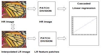
Fig. 1. Flow of cascaded linear regression framework
B. Pseudo code For Cascaded Linear Regression Algorithm
The Pseudo code for cascaded linear regression algorithm for training phase is given below,
Input: , image patch size √d x√d
for t=1 to T
do
{

Apply k-means to obtain cluster centres 
for i = 1 to c
do
{
compute A and b.


update the values of A and b in  .
.
}
end for
}
end for
The output of this training phase is  and cluster centroid
 .
.
C. SERF Image Super-Resolver
This section deals with cascaded linear regression based SERF image. The process starts by converting color image from the RGB space into the YCbCr space where the Y channel represents luminance, and the Cb and Cr channels represent the chromaticity. SERF is only applied to the Y channel. The Cb and Cr channels reflect G and B channels of the interpolated LR image.
D. SERF Implementation
To extract the high frequency details from each patch by subtracting the mean value from each patch as feature patch denoted as  . Since the frequency content is missing from the initially estimated image patches, the goal of a series of linear regression is to compensate for high frequency detail (4),
 (4)
(4)
To diminish the error between HR feature patch and the estimated feature patch, it is normal that the regression output should be small. Hence, by putting the constraint on regularization term to (4), the output is,
 (5)
(5)
Where, λ is the regularization parameter.
t – Denotes the number of regression stages.
 – denotes the feature extractor.
β and λ are set to 1 and 0.25.
A closed-form solution for equation (5) can be computed by making the partial derivative of equation (5) equal to zero.
In testing phase, for a given LR image, bicubic interpolation is applied to up sample it by a factor of r. This interpolated image is divided into M image patches. Feature patches are calculated by subtracting the mean value from each image patch. At the tth stage, each feature patch is assigned to a cluster l according to the Euclidean distance. To obtain the feature subsequently, linear regression parameters are applied to compute the increment. Concurrently, the feature patch is updated using,
 (6)
(6)
After passing through T-stages, reconstructed image patches are obtained by adding mean value to the final feature patches. All the reconstructed patches are then combined with the overlapping area and then averaged to generate the original HR image.
E. Pseudo code For SERF Image Super-Resolver Algorithm
The pseudo code for SERF image super-resolver algorithm is as follows:
Inputs: Y, a, r, 
for t=1 to T
do
{
Adapt each patch cluster to a cluster.
Compute .
.
Update the values of A and b in 
}
End for
The output will be the High Resolution image (HR).
The simulation of the SERF image super-resolver is done by using MATLAB R2013a for various images. The LR image is read from image folder and is processed using the algorithms explained before. The output HR image is taken after regression stages. The implementation is done by considering many reference images. The colour image (RGB) is first converted into YCbCr space, where Y channel represents luminance. Cb and Cr are simply copied from the interpolated LR image. The number of cluster size is 200. Image patch size 5 x 5 and magnification factor is set to 3.
|
|
|
|
|
a)LR input |
b)HR input |
(c)Zooming result |


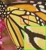
Fig.2. SERF Result under Magnification Factor 3
|
|
|
|
|
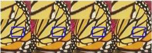
a)LR input |
b)HR output |
c)zooming result |


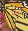
Fig.3. SERF Result under Magnification Factor 2
|
|
|
|
|
a)LR input |
b)HR output |
c)zooming result |


Fig.4. SERF Result under Magnification Factor 1
(a) (b) (c) (d)
(e) (f) (g) (h)
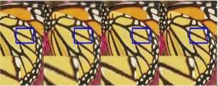
Fig.5. Comparisons Results–Butterfly (a) ground truth image (original size is 256 Ã- 256); (a)super-resolution results of (b) SRCNN, (c) ScSR, (d) Zeyde’s, (e) ANR, (f) BPJDL,(g) SPM, and (h) SERF.
Zeyde’s [5] method gives noiseless image, but texture details are not well reconstructed as shown Figure (d). The BPJDL [14] methods generate sharper edges when compared to other methods as shown Figure (f). Figure (h) shows the zooming results of SERF method that performs well for both reconstruction and visual artifacts suppression.
TABLE I:PSNR AND SSIM VALUES UNDER MAGNIFICATION FACTOR OF 1, 2 AND 3.
|
Magnification Factor |
PSNR |
SSIM |
TIME(s) |
|
3 |
29.0775 |
0.839 |
0.4323 |
|
2 |
30.5 |
0.812 |
0.4000 |
|
1 |
38.4 |
0.798 |
0.3870 |
TABLE II:PSNR AND SSIM VALUES UNDER MAGNIFICATION FACTOR OF 3 FOR TESTING IMAGES.
|
S.NO |
IMAGES |
PSNR |
SSIM |
TIME(s) |
|
1 |
Baboon |
23.63 |
0.532 |
0.3115 |
|
2 |
Baby |
35.29 |
0.906 |
0.4148 |
|
3 |
Butterfly |
26.87 |
0.883 |
0.2018 |
|
4 |
Comic |
24.32 |
0.755 |
0.2208 |
|
5 |
Man |
28.19 |
0. 778 |
0.5468 |
|
6 |
zebra |
29.09 |
0.839 |
0.4324 |
For magnification factor of 3, SERF outplays ScSR method by an average PSNR gain of 0.43dB, Zeyde’s [5] method by 0.37dB, ANR [15] by 0.44dB, BPJDL [14] method by 0.23dB and the SPM [7] method by 0.16dB. SERF gives average SSIM value of 0.8352 and it is fastest method compared to existing methods (TABLE III).
TABLE III: PSNR AND SSIM VALUE COMPARISON OF SERF METHOD WITH EXISTING METHODS UNDER MAGNIFICATION FACTOR OF 3.
|
EXISTING METHODS |
PSNR |
SSIM |
TIME(s) |
|
ScSR [4] |
23.69 |
0.8835 |
7.27 |
|
Zeyde’s [5] |
23.60 |
0.8765 |
0.06 |
|
ANR [15] |
24.32 |
0.8687 |
0.02 |
|
BPJDL [14] |
24.17 |
0.8890 |
17.85 |
|
SPM [7] |
24.63 |
0.8982 |
0.74 |
|
SERF |
29.0775 |
0.8352 |
0.23 |
SERF has few parameters to control the model, and results in easy adaption for training a new model when the experimental settings, zooming factors and databases were changed. The cascaded linear regression algorithm and SERF image super-resolver has been simulated in MATLAB2013a. SERF Image super-resolver achieves better performance with sharper details for magnification factor up to 3. This model reduces the gaps of high-frequency details between the HR image patch and the LR image patch gradually and thus recovers the HR image in a cascaded manner. This cascading process promises the convergence of SERF image super-resolver. This method can also be applied to other heterogeneous image transformation fields such as face sketch photo synthesis. Further this algorithm will be implemented on FPGA by proposing suitable VLSI architectures.
REFERENCES
[1] W. Freeman, E. Pasztor, and O. Carmichael, “Learning low-level vision,” International Journal of Computer Vision, vol. 40, no. 1, pp. 25-47,2000.
[2] J. Sun, N. Zheng, H. Tao, and H. Shum, “Image hallucination with primal sketch priors,” in Proceedings of IEEE Conference on Computer Vision and Pattern Recognition, 2003, pp. 729-736.
[3] Q. Wang, X. Tang, and H. Shum, “Patch based blind image super resolution,” in Proceedings of IEEE international Conference on Computer Vision, 2005, pp. 709-716.
[4] J. Yang, J. Wright, T. Huang, and Y. Ma, “Image super-resolution via sparse representation,” IEEE Transactions on Image Processing, vol. 19,no. 11, pp. 2861-2873,2010.
[5] R. Zeyde, M. Elad, and M. Protter, “On single image scale-up using sparse-representations,” in Proceedings of Curves and Surfaces, 2012, pp. 711-730.
[6] X. Gao, K. Zhang, D. Tao, and X. Li, “Joint learning for single-image super-resolution via a coupled constraint,” IEEE Transactions on Image Processing, vol. 21, no. 2, pp. 469-480, 2012.
[7] K. Zhang, X. Gao, D. Tao, and X. Li, “Single image super-resolution with multiscale similarity learning,” IEEE Transactions on Neural Networks and Learning Systems, vol. 24, no. 10, pp. 1648-1659, 2013.
[8] G. Freedman and G. Fattal, “Image and video upscaling from local selfexamples,” ACM Transactions on Graphics, vol. 28, no. 3, pp. 1-10, 2011.
[9] K. Zhang, D. Tao, X. Gao, X. Li, and Z. Xiong, Learning multiple linear mappings for efficient single image super-resolution,” IEEE Transactions on Image Processing, vol. 24, no. 3, pp. 846-861, 2015.
[10] K. Kim, D. Kim, and J. Kim, “Example-based learning for image super resolution,” in Proceedings of Tsinghua-KAIST Joint Workshop Pattern Recognition, 2004, pp. 140-148.
[11] K. Zhang, D. Tao, X. Gao, X. Li, and Z. Xiong, “Learning multiple linear mappings for efficient single image super-resolution,” IEEE Transactions on Image Processing, vol. 24, no. 3, pp. 846-861, 2015.
[12] M. Yang and Y. Wang, “A self-learning approach to single image super resolution,” IEEE Transactions on Multimedia, vol. 15, no. 3, pp. 498-508, 2013.
[13] K. Kim and K. Younghee, “Single-image super-resolution using sparse regression and natural image prior,” IEEE Transactions on Pattern Analysis and Machine Intelligence, vol. 32, no. 6, pp. 1127-1133, 2010.
[14] H. He and W. Siu, “Single image super-resolution using gaussian process regression,” in Proceedings of IEEE Conference on Computer Vision and Pattern Recognition, 2011, pp. 449-456.
[15] R. Timofte, V. Smet, and L. Gool, “Anchored neighborhood regression for fast example-based super-resolution,” in Proceedings of IEEE Conference on Computer Vision, 2013, pp. 1920-1927.
[16] J. Yang, Z. Lin, and S. Cohen, “Fast image super-resolution based on in-place example regression,” in Proceedings of IEEE Conference on Computer Vision and Pattern Recognition, 2013, pp. 1059-1066.
[17] C. Dong, C. Loy, K. He, and X. Tang, “Learning a deep convolutional network for image super-resolution,” in Proceedings of European Conference on Computer Vision, 2014, pp. 184-199.
[18] C. Dong, C. Loy, K. He, and X. Tang, “Image super-resolution using deep convolutional networks,” IEEE Transactions on Pattern Analysis and Machine Intelligence, DOI:10.1109/TPAMI.2015.2439281, 2015.
[19] P. Viola and M. Jones, “Robust real-time face detection,” International Journal of Computer Vision, vol. 57, no. 2, pp. 137-154, 2004.
Cite This Work
To export a reference to this article please select a referencing stye below:
Related Services
View all


DMCA / Removal Request
If you are the original writer of this essay and no longer wish to have your work published on UKEssays.com then please click the following link to email our support team:
Request essay removal