Macroeconomic Fundamentals Lecture
Chapter Summary
Welcome to the next lesson of this module where we will cover the topic of macroeconomic fundamentals.
The chapter sheds light on a fundamental set of economic notions and instruments that are crucial to understand contemporary economic relations at a global level.
Firstly, the chapter will present a graphical analysis of market supply and demand, then moving onto explaining the concepts of aggregate supply and demand. It further introduces the concept of Gross Domestic Product (G.D.P.), as well as some of its basic constituents and derivations to develop an understanding.
The chapter discusses inflation which constitutes a macroeconomic measurement that reflects the general increase of the overall price level associated with a given economy. This is then finished off with investigating the determinants of national income and the circular flow of the income model.
Goals for this chapter:
To understand the macroeconomic fundamentals and concepts used
1. Introduction
The global financial crisis of 2007 - 2008 and the corresponding impact on the global economy has drawn significant attention to the pressing macroeconomic questions that currently affect the world’s population. In the aftermath of the global systemic shock, macroeconomic fundamentals have come to the centre of the global economic debate on policy making. These fundamentals thus constitute a global and pressing topic of the utmost importance, as world economic growth is highly dependent on existing market mechanisms and structures that have a leveraging impact on economic growth, although these mechanisms are strongly sensitive to the negative impact of global financial disruptions (Blanchard, 2009).
The present document is intended to provide a succinct introduction to the topic of global macroeconomic fundamentals, and corresponding nuclear topics. The present document thus sheds light on a fundamental set of economic notions and instruments that are crucial to understand contemporary economic relations at a global level.
2. Basic demand and supply: a graphical analysis
In standard economics, the marketplace typically has two dimensions: market demand and market supply. The former is related to the needs of economic agents in relation to a set of goods and services they need in order to conduct their lives in society, and against which they are willing to pay a given established market price; while the latter refers to the set of goods and services effectively provided by the market place in exchange for the corresponding applicable market prices for the produced goods and services.
Each of these opposing dynamics might be portrayed by a specific schedule: the demand curve and the supply curve. Each of these curves is related to a specific good or service associated with a specific market. Taking into consideration that different prices might elicit distinct responses from both buyers and sellers (individually considered), two different schedules can be described: the demand curve and the supply curve (Krugman, et al., 2011).
2.1. Market demand
Figure 1. The demand curve for a single product or service [D(0)].
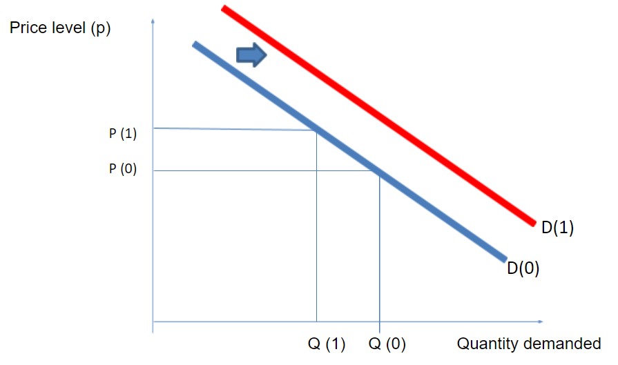
In Figure 1, the demand curve for a given good or service depicts the different price /quantity combinations consumers are willing to pay for in order to consume the said good or service. As expected, the higher the price, the lower the quantity demanded by consumers, as prices are negatively correlated with demanded quantities. If prices rise from p(0) to p(1), the quantities demanded fall from q(0) to q(1). This refers to changes along the curve (curve shifts from D(0) to D(1) will be dealt with at the end of the section).
Need Help With Your Economics Essay?
If you need assistance with writing a economics essay, our professional essay writing service can provide valuable assistance.
See how our Essay Writing Service can help today!
2.2. Market supply
Figure 2. The supply curve for a single product or service [S(0)].
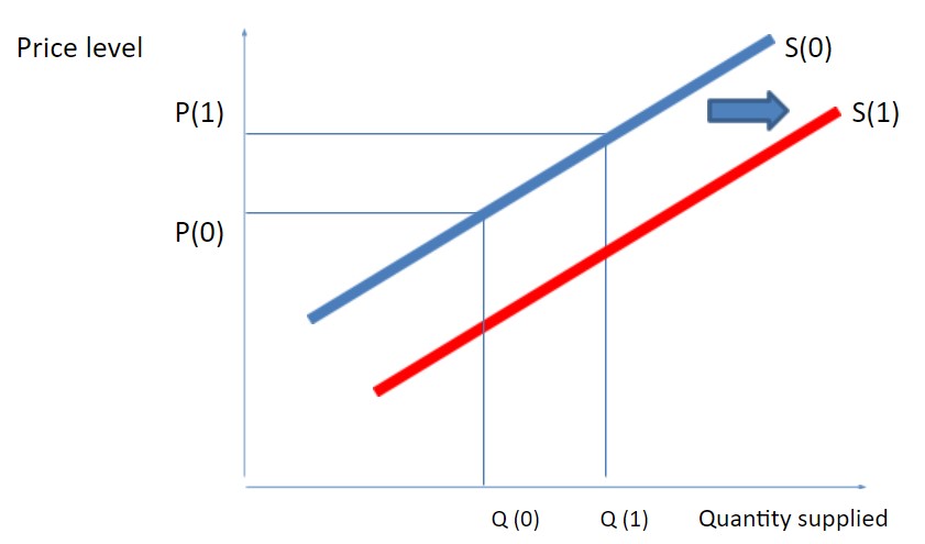
In Figure 2, the supply curve for a given good or service depicts the different price/quantity combinations producers willing to get paid for in order to produce a given good or service. As expected, the higher the price, the higher the quantity supplied by business producers, as prices are positively correlated with supplied quantities. If prices rise from p(0) to p(1), the quantities demanded also rise from q(0) to q(1) (curve shifts from S(0) to S(1) will be dealt with at the end of the section).
2.3. Market equilibrium
In any given market for a specific good or service, the market transaction takes place when both these schedules occur simultaneously, i.e., when both the demand and the supply curve intersect. This point of intersection is called the market equilibrium point, and this point is characterised by a single market price (at equilibrium) and a single quantity (at equilibrium). This equilibrium point thus presents two coordinates (price, quantity) that satisfy both consumers and producers alike. The market equilibrium is depicted in Figure 3 (Sloman, et al., 2012).
Figure 3. Market equilibrium for a specific good or service.
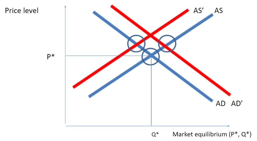
It is important to distinguish between movements along a given curve or shifts in each curve. Movements along a given curve essentially portray the different combinations between price and quantities that the consumer (or the producer) are willing to consume (produce). Shifts associated with a given curve typically describe an exogenous event or shock that took place and structurally changed the relationship between price and quantities consumed (produced). For example, in Figure 1, if there is a positive wealth effect faced by a given consumer (e.g. she/he earns a higher wage), then for any given price, the quantities demanded increase. In Figure 2, if there is a positive cost shock (e.g., energy prices go down), then for any given price, the quantities supplied are higher (as producers can now produce a greater quantity at any given price). It should be observed that economic shocks can be either positive or negative, and the corresponding impact is different whether it applies to the demand side or to the supply side. For example, the circles described in Figure 3 point to different equilibrium points when there are shifts in either the demand curve (from AD to AD’) or the supply curve (from AS to AS’).
These mechanisms are usually applicable to specific markets for goods or services, but this economic reasoning can be extended to global macroeconomic issues, as the next section clearly illustrates.
3. Aggregate demand and aggregate supply
The present section first introduces the concepts of aggregate demand (section 2.1.) and aggregate supply (section 2.2.); it further introduces the concept of Gross Domestic Product (G.D.P.), as well as some of its basic constituents and derivations (section 2.3.), it finally introduces the concept of inflation.
3.1. Aggregate demand
There are certain macroeconomic concepts that are fundamental to understand the way the global economy works. Aggregate demand is a fundamental macroeconomic concept that essentially depicts the relationship between the aggregate price level in any given economy and the total quantity of joint (i.e., aggregate) output demanded by a set of economic agents comprising business firms, households, the government, and by other economic agents located in the rest of the world.
Prior to introducing the concepts herein exposed, it is important to detail a basic taxonomy of the categories of economic agents typically involved in macroeconomic issues. The following paragraphs illustrate these generic/broad categories (Sloman, et al., 2012) (Mishkin, 2015).
Business firms typically constitute an organised form of production structures that produce goods and/or services that cater to their certain consumers in their corresponding industries. These business firms are typically profit-oriented, seeking to optimise profits for their corresponding shareholders. These organised production structures typically use a set of production inputs in order to produce the firm’s products and/or services. Some of the inputs used in a business firm’s transformative processes include: human capital, financial capital, buildings and plant factories, transportation equipment, intellectual property rights, etc.
Households are typically constituted by a person or a set of persons that occupy a housing unit, collectively sharing household resources, financial or otherwise. These households are consumers of the products and/or services produced by business firms, but they might also consume products and/or services provided by the government and/or foreign entities (e.g., external business firms incorporated in other countries that export to the country where the household is located). These households critically depend on either incomes (from one or multiple different sources), and/or their wealth, in order to fund their household purchases of goods and/or services.
The government determines public economic policy, all the while exercising macroeconomic executive power that influences the country’s economy. Accordingly, the government, in the fulfillment of the corresponding duties, needs to buy goods and/or services necessary to the fulfillment of its duties towards its citizens (e.g., it needs to buy machinery to build roads and bridges). In order to do so, the government then goes to the marketplace, but it should be pointed out that this governmental economic agent has significant market power, as the pecuniary amount (and even the volume) of its purchases is typically quite considerable.
Aggregate demand thus constitutes an economic measurement reflecting the sum of all final goods and services produced within a given economy, as expressed by the total amount of money exchanged for those goods and services (in theory, it reflects price P times quantity Q, summed up for all the complete range of goods and services produced and exchanged by a given economy). It should be taken into consideration that this economic indicator is measured using market values that reflect current prices for these goods and services. Therefore, aggregate demand typically represents the total amount of economic output considered at a certain overall price level. Lastly, it should also be noted that this important economic measurement does not possess any specific economic welfare implication; but instead constitutes an accounting and economic tally for the complete set of goods and services produced within a given economy, as these are necessarily consumed by the three types of economic agents above mentioned described within a given economy - business firms, households, and the government. These economic agents thus constitute the main purchasers[1] of the goods and services produced by the economic system (Mishkin, 2015).
Moreover, it should be pointed out that there are two essential reasons why aggregate demand constitutes an important macroeconomic concept. First, aggregate demand is one of the most observed macroeconomic indicators simply because this measurement signals variation throughout time and provides a solid basis for understanding how the productive dimension of the underlying economy is evolving in the said time interval. Second, the concept of aggregate demand is also quite fundamental to policy makers simply because these regulatory agents have to monitor the macroeconomic performance of the economy, and be able to intervene accordingly (should a given economic state prompt a regulatory action). These two reasons are quite important in times of economic crisis, where economic activity typically slumps, and when policy makers generally have to intervene in the economy, either through fiscal policy, or through monetary policy, or both. This policy making intervention is therefore crucial in order to stimulate economic activity when the said activity is slumping. The proper monitoring beforehand of the historical evolution of aggregate demand might thus be important in times of economic crises, in order to assess how the general economy is faring, and when policy intervention is warranted (Mishkin, 2015).
Lastly, aggregate demand is at the basis of the aggregate demand curve, which takes into consideration the total impact in aggregate demand from a variation in the overall price level. That is, recognising that the price level might influence aggregate demand, the higher the price, the lower the level of aggregate demand. Therefore, the relationship between the aggregate demand curve and the overall price level is a negative one, insofar as higher prices lead to a decreased demand for goods and services in the economy. The negative relationship between aggregate demand and the overall price level is depicted in the aggregate demand curve depicted in Figure 4.
Figure 4. The aggregate demand curve AD.
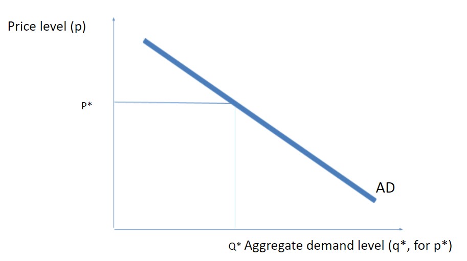
In Figure 4, it is quite noticeable that the higher the price level, the lower the total quantity associated with aggregate demand (labelled AD in the negative schedule), simply because, at higher prices, the demand side economic agents (e.g., business firms; households; the government) consume less, all other variables remaining equal (“ceteris paribus” condition).
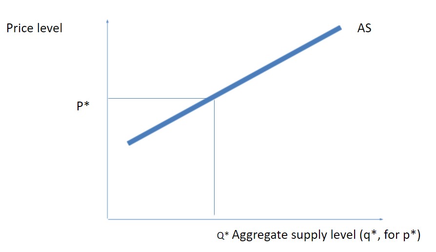
3.2 Aggregate supply
Reciprocally, aggregate supply constitutes an economic measurement reflecting the sum of all final goods and services produced and supplied within a given economy, as expressed by the total amount of money exchanged for those goods and services. Aggregate supply thus reflects the economic activity occurring on the productive dimension of the economy (e.g., in the business firms providing goods and services to the economy) (Mishkin, 2015).
Taking into consideration the above mentioned reasoning depicting the association of these economic measurements with the overall price level, the aggregate supply curve thus depicts the relationship between the economy’s aggregate supply of final goods and services produced by the suppliers that are willing to supply the market, and the overall price level in the economy. In the specific case of the aggregate supply curve, this relationship is positive sloping, as a higher price level induces producers to increase their production of goods and services as higher prices increase turnover and profits; while a lower price level induces producers of goods and services to produce a much lower volume of production, due to depressed turnover and profits. That is, producers of goods and services prefer a higher overall price level (in detriment of lower overall price level) simply because they benefit more when the prices are higher. This happens because profits per unit of output are equal to the price per unit of output minus the production cost per unit involved in the output’s production. Taking into consideration that most of the costs in the short run are fixed (e.g., the wages of salaried workers is typically constant in the short term), then profits per unit of output produced greatly increase when prices increase (this happens simply because wage growth is inexistent in the short run, leading to higher profits to the producer). Figure 5 illustrates an upward sloping aggregate supply curve (Mishkin, 2015).
Figure 5. The aggregate supply curve AS.
3.3. Aggregate market equilibrium
When comparing both Figures 4 and 5, it should be pointed out that, contrary to the previously mentioned case where the aggregate demand curve was downward sloping, the aggregate supply curve is upward sloping. Moreover, the overall market equilibrium occurs when the two curves intersect (as in the previously described simple demand and supply schedules for a specific good or service). When the two curves meet, this intersection point reveals the optimal combination of overall prices and quantities produced (P*,Q*) that satisfy both schedules.
That is, the market equilibrium in the overall economy results from the intersection of the aggregate demand curve and the aggregate supply curve, as evinced in Figure 6 (Mishkin, 2015).
Figure 6. Equilibrium between aggregate demand and aggregate supply
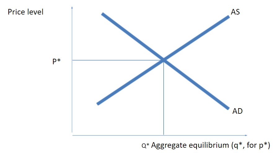
In Figure 6, AD stands for aggregate demand and AS stands for aggregate supply, while Q* refers to the total aggregate output produced in the economy at the overall P* price level. .
Lastly, it should also be pointed out that the shape for the aggregate supply curve in the long run is vertical (and not upward sloping as AS in Figure 6). This is because, in the long run, each and every producer of goods and services would see any profit accruing from a potential price increase (decrease) entirely neutralised by a correspondingly increase (decrease) in production costs, so that profits per unit produced would remain neutral. In other words, halving or doubling prices in the economy would have no effect on the economy’s aggregate output, as changes in the aggregate price level would bear no effect on the overall quantity of aggregate output supplied by producers of goods and services in the economy (the reasoning in this paragraph only applies to the aggregate supply side) (Mishkin, 2015).
BOX 1. AGGREGATE DEMAND AND AGGREGATE SUPPLY
IN A POST-CRISIS ENVIRONMENT
The U.S. economy has been slowly recovering from a most severe financial and economic recession in the aftermath of the 2007-2008 ‘Subprime’ crisis. Accordingly, the pace of the economic recovery in the U.S.A. has been less vigorous than might have been desired or even expected, as U.S. national income has been quite slow to recover from the global financial shock.
The main culprit associated with a slowdown in aggregate demand is related to the negative wealth effect brought about by the implosion of the U.S. real estate and credit derivatives markets, which led to significant losses for households, business firms, and even the government. In the context of a post-crisis environment, households are still deleveraging from excessive debt, businesses are still quite reluctant to invest, and governments have accumulated excessive public debt in the aftermath of the crisis.
It should be observed that, in the context of a post-crisis environment, central bank interest rates have been nearly at zero, which signals that credit is fundamentally ‘cheap’, which should stimulate aggregate demand. Nevertheless, the global economy has been slow to pick up.
It should be further noted that a slump in aggregate demand ended up having an impact on aggregate supply as well, once the economic shock’s time lag is taken into consideration as well. That is, once producers observed that aggregate demand slumped in the aftermath of the global systemic shock, they adjusted their expectations so as to also be able to accommodate the said shock, lowering their production outlays, and reducing their use of organisational inputs accordingly, thus indirectly promoting unemployment. Through this chain of economic events, an aggregate demand shock turned into an aggregate supply shock that led to a diminishment of economic output in the global economy and the Great Recession of 2007 - 2008.
Source: (Yellen, n.d.).
The following section presents the macroeconomic concept of G.D.P., based on the previously presented economic concepts.
4. G.D.P. - its assessment, components and different variations
The present section illustrates how G.D.P. can be assessed through three different sources (sub-section 4.1.), what are G.D.P.’s components, G.D.P.’s components (sub-section 4.2), as well as different variations thereof (sub-section 4.3.).
4.1. The assessment of G.D.P.
Gross Domestic Product (G.D.P.) is defined as the total value of all final goods and services produced in a given economy during a given period (from a national accounts perspective, this is usually considered to be a year).
There are essentially three ways through which a given country’s G.D.P. numbers can be estimated. The first estimation method addresses the surveying of producers of goods and services in order to assess the overall value of their production in each individual case, and adding up the total production value of all final goods and services across the economy. In this specific case, it should be observed that, in order to avoid multiple accounting of the same good throughout the production process involving several business firms, this tally only takes into consideration the production of final goods and services across the economy. That is, the consumption of intermediate goods - those that stand as inputs to other producers - stands excluded from this tally, in order to avoid accounting for the said product throughout a given industry’s production chain.
A second estimation method addresses tallying the total spending on final goods and services consumed in the economy. Specific economic agents spend their income (or part of their wealth) in acquiring goods and services in the marketplace. This specific method comprehensively adds aggregate spending on the amount of goods and services produced domestically in the economy. For example, the total number of households in any given economy collectively possesses a significant purchasing power (jointly considered). That is, these numbers can be tallied in order to account for G.D.P. through aggregate spending (instead of production, as in the first estimation method).
A third estimation method is based on aggregate income earned by economic agents established in the economy. For example, the factors of production employed by business firms in the above-mentioned transformation processes are typically provided by households, namely the human capital (e.g., individual workers) employed in these business firms. That is, business firms employing human capital typically pay a share of their earnings accruing from their business activities to households, through the payment of individual wages. Accordingly, a third method for assessing G.D.P. addresses the aggregate sum of total factor income earned by a given economy’s households and other economic agents in the economy (Sloman, et al. 2012) (Krugman, et al., 2011).
4.2. G.D.P.’s components
As previously presented, G.D.P. is a nuclear economic concept that can nevertheless be broken in smaller components. For example, and adopting the expenditure method of estimating G.D.P., the latter economic measurement concepts adds up all the categories associated with different types of expenditure, more specifically: i) personal consumer expenditure (C); investments (I); government expenditure (G); and exports (X). Adding these components, and deducting for the amount of imports (I), G.D.P. is thus given by the following equation:
G.D.P. = C + G + I + X - M, for a given civil year t (1)
In this case, personal consumption expenditures refer to expenditures related to households (families and individuals); government expenditures refer to the expenditures faced by the government (considered as a sole economic agent with massive purchasing power); investments refer to the acquisitions destined to replenish capital instruments servicing production; exports refer to expenditures realised by foreign economic agents buying specific products and/or services in the local economy; and, lastly, imports refer to the local economy’s acquisitions of good and/or services produced in other foreign markets (often, G.D.P. uses the concept of net exports to refer to the difference between exports and imports, thus substituting the terms X - M by a single variable denoting external trade’s net effect on equation (1).
This is the standard way of presenting G.D.P.’s components in the national accounts (Sloman, et al., 2012).
4.3. G.D.P.: some important conceptual variations
It should be observed that G.D.P. is an important economic measurement concept that can be adapted to many variants that shed light on specific sub-concepts (Sloman, et al., 2012) (Krugman, et al., 2011).
For example, an important variation addresses the difference between nominal G.D.P. and real G.D.P. In essence, nominal G.D.P. measures total production of goods and services throughout the economy in a given year; accordingly, this sub-concept does not take single out the existence of inflation (this important economic concept will be presented in the next sub-section), as variations in prices are also incorporated in nominal G.D.P. Real G.D.P. takes into consideration the measurement of G.D.P. using prices that were applicable in a given base year in the past. That is, real G.D.P. could be measured using quantities associated with year t, but using prices associated with year t - n (for example, a measurement of real G.D.P. for 2016 could be estimated using prices associated with, say, the base year of 2000). The essential difference between these two concepts addresses the fact that real G.D.P. effectively captures variations in quantities produced from one year to the following, therefore eliminating increases in nominal G.D.P. that might be attributed to an increase in prices.
Another important variation addresses the estimation of G.D.P. using population numbers. When comparing amongst countries with distinct demographic, geographical, economic and social characteristics, it might be more useful to refer to G.D.P. per capita (instead of using G.D.P. in absolute values). The said concept is duly obtained by dividing G.D.P. at current market prices in absolute terms (as above presented) by the country’s general population. This therefore indicates the amount of the national production that is directly attributable to each member of the general population. This economic measurement indicator is quite useful in the formulation of public policies, because through the measurement of the level of total economic output in relation to the country’s population, this reflects visible economic changes in the total economic well-being of the said population. Nevertheless, it is necessary to observe that this economic measurement does not constitute an economic welfare measurement whatsoever. G.D.P. per capita is thus a powerful and elucidative macroeconomic indicator of sustained economic development. Notwithstanding the fact that G.D.P. per capita does not directly measure economic development, it nevertheless constitutes quite an important assessment for developmental and economic sustainable development.
Another G.D.P. variant has to do with the measurement in different countries that have different legal tenders. When comparing G.D.P. numbers for different countries, the purchasing power for G.D.P. per currency unit is quite different in multiple countries (for example, £1 in the U.K. does not have the same purchasing power as €1 in the Euro Area, as foreign exchange rates have to be taken into consideration). Accordingly, when establishing comparisons involving G.D.P. estimates in different countries possessing different currencies, G.D.P. estimates can be adjusted in order to accommodate currency exchange movements. This is the purchasing power G.D.P., whereby these economic estimates are converted into a common currency at a given purchasing power parity rate. Accordingly, this mechanism allows, under a parity exchange rate, to compare G.D.P. estimates in multiple countries.
Lastly, it should be observed that the measurement of national output is not as straightforward as might be supposed, as there are several statistical problems underlying these measurement activities. First, if a household, for example, hires an employee to cater for house cleaning activities, then this item is categorised as an expenditure associated with the said household. If, however, these household’s cleaning activities are performed by the various family members associated with the said household, then these activities are not tallied in the G.D.P. numbers, although these activities are bound to take place (in the end, the household needs to be cleaned, regardless of whether this activity might be included in the country’s G.D.P. estimates).
Another major issue associated with the measurement of G.D.P. is related to the fact that the economy also encompasses what might be termed the ‘underground’ economy. This sector essentially consists of undeclared transactions and/or illegal economic transactions (the former address transactions of legally tradable goods in tax-evading circumstances; while the latter addresses transactions of goods and/or services that are themselves illegal). This poses a tremendous problem for national statistical authorities, as G.D.P. might be seriously under-estimated because the ‘underground’ economy is not duly accounted for, thus evading the control of policy makers, tax authorities, and regulators (Sloman, et al., 2012).
BOX 2. ADVANTAGES AND DISADVANTAGES OF G.D.P.
G.D.P. estimates are quite relevant in policy making, insofar as they provide an overall picture of the macroeconomic dynamics associated with a given economy. That is, G.D.P. numbers typically reflect the major economic trends impacting a given economy, notwithstanding the existence of some statistical measurement problems that might affect the economic measurement indicator’s computation (please see main text above).
Where the main advantages of using this economic indicator are concerned, it should first be pointed out that its use provides quite a simple and universal estimate of the macroeconomic state of the underlying economy; further, this indicator has also been extensively used in a policy making context for a very long time, so that there are historical time series that portray the state of macroeconomics in a historical perspective; moreover, the use of these series allows for national and international comparisons across time, thus providing a historical analysis of a single country or a group of countries across time, as this indicator is quite reliable over the long-run; further, these international estimates are also fairly stable over time as to their object of study (the measurement of macroeconomic activity); lastly, these estimates also positively correlate with other alternative measurement concepts that capture the same type of definition (or a derivation thereof).
Where the disadvantages are concerned, there are some related economic phenomena that are not acknowledged in the G.D.P. concept. For example, G.D.P. estimates do not account for the impact of negative externalities on economic growth (e.g., pollution, or CSR incidents); the transaction of illegal goods is also not accounted for (notwithstanding the size and volume of some of these transactions in the economy); health- and leisure-related questions and issues are also not given appropriate economic treatment in these national estimates; finally, there are also multiple methodological/statistical problems and issues that merit further attention (e.g., estimations on the distribution of income and wealth, etc.); lastly, these estimates do not constitute an economic measurement of the economic welfare of a given country nor of its citizens.
Nevertheless, it should be observed that these estimates are the best possible macroeconomic and statistical indicators, as they constitute a transversal platform for having a basic understanding of how a given country’s macro economy works.
Source: Krugman Sloman, et al. (2012); Krugman, et al. (2011).
5. Inflation
As described in previous sections, prices are dynamical over time, as they change to accommodate different economic circumstances. When prices rise, they might rise consistently over time, or they might rise non-persistently. When the rise in prices constitutes a persistent trend, the economy may be subjected to inflationary pressures - inflation, for short.
Inflation thus constitutes a macroeconomic measurement that reflects the general increase of the overall price level associated with a given economy. It should be pointed out that this overall trend may be captured by a variable or proxy thereof that encompasses the overall trend in price dynamics. For example, inflation might be typically represented by an inclusive price index, such as a consumer price index. This index represents a vast majority of individual prices in the economy, rising (or falling) collectively, as opposed to a sub-set of prices that rise in isolation, while the remaining majority does not (e.g., this might be the case of rising fuel prices, which might be rising when non-fuel prices are quite stable) (Lipsey and Chrystal, 2015).
Inflation is thus a macroeconomic variable that is best expressed as a variation. That is, inflation is best expressed as an inflation rate that is typically periodical in nature (e.g., the inflation rate might be expressed annually). The inflation growth rate thus measures the increase in the overall price structure in the economy, as measured by an economic index. Nevertheless, the inflation rate might also be expressed as a rate related to a shorter intra-annual period of time (e.g., quarterly).
Need Help With Your Economics Essay?
If you need assistance with writing a economics essay, our professional essay writing service can provide valuable assistance.
See how our Essay Writing Service can help today!
Persistent inflation is typically a very noxious economic phenomenon, as it erodes the purchasing power of economic agents. That is, persistent inflation corrodes economic growth and the expenditure outlay of economic agents, as it can greatly reduce the amount of goods and/or services a given amount of income can buy in the market place. When inflation is high and persistent - as in the case of two-digit annual inflation growth rates - the majority of economic agents see their purchasing power diminish quite strongly, as the same amount of, say, monthly wages acquire a lesser volume of goods and services (assuming that the set of expenditures remains constant over time, i.e., the composition of expenditures is the same over the scrutinised period) (Lipsey and Chrystal, 2015).
On the other hand, persistently high inflation is self-compounding, insofar as unstable inflation is typically associated with ever greater increases in the inflation rate in the near future. That is, for example, double digit inflation tends to be self-compounding, as chronic inflation perpetuates itself in increasingly higher numbers (i.e., a 20% annual inflation rate can quite rapidly turn into an inflation rate of 40% or 50% or more, should this problem not be immediately tackled by the relevant economic authorities) (Balderston, n.d.). That is, chronic inflation rates can easily turn into a hyperinflationary shock, through the erosion of national income and wealth, as the historical example provided in Box 3 clearly demonstrates.
BOX 3. THE GERMAN HYPERINFLATION OF THE 1920’S
German hyperinflation was a severe economic phenomenon that originated in the aftermath of the First World War, through the decision that was undertaken in July and August of 1914, suspending the standard of gold convertibility involving the Deutsche Mark and the corresponding parity related to gold reserve requirements. Typically, hyperinflationary phenomena tend to be quite serious, as their onset reveals the inability of economic authorities to deal with this pressing problem. For example, German wholesale prices more than doubled throughout the years associated with the First World War. By February of 1920, the increase in relation of the base year of 1913 prices was about 17% and stabilised until May of 1921. After May, inflation rates started increasing, and, until June of 1922, the average monthly inflation rate was 13.5 %; thereafter, in the following 12 months, the inflation rate further reached 60%, and, quite suddenly, between June and November of 1923, the inflation rate reached a staggering rate of 32’700%, which is roughly equivalent to about 20% per cent per day (!). This essentially means that prices in stores, for example, had to be adjusted throughout the business day, in order for producers to avoid selling their wares at a loss. The end result was that, in November of 1923, the foreign exchange rate involving the U.S.D. -Deutsche Mark stabilised at about one million millionth of its pre-inflationary 1913 dollar exchange rate, although, from a technical point of view, only the period after June 1922 is considered to be ‘hyperinflationary’ - a state where inflation rates soars to more than 50% per month. It goes without saying that this period was marked by great economic uncertainty, leading economic agents to be heavily dependent on adjusting their economic activities on a daily basis in order to accommodate fast changing prices in the economy.
Source: Balderston (n.d.)
In order to address this pernicious economic phenomenon, central banks have had an aggressive posture in relation to combatting inflation. Central banking institutions are the proper governmental agency in charge of conducting monetary policy in a given country (or set of countries, such as the Euro Area). In the context of the post-crisis environment, central banks have added fundamental financial stability functions, although historically, the main task of central banks addressed price stability functions[2], simply because high and persistent inflation ended up corroding economic growth, through the erosion of income and wealth’s purchasing power. Accordingly, central banking institutions such as the Bank of England have implemented a nuclear monetary policy rule upholding price stability, choosing an acceptable limit to inflation of around 2%. This target is considered an acceptable and tolerable rate of inflation, a level above which central banks start to intervene in the financial markets in order to curb inflation (Bank of England, 2017).
6. Determinants of national income
There are multiple determinants that might condition the measurement of national income in a given country. These determinants can be comprehensively categorised as follows (Economic Concepts, n.d.):
i) the joint stock of factors of production: the proper combination of factors of production (either in terms of quantity and/or the quality of these factors) constitutes a critical success factor that determines the national income of a given country. The individual factors of production in question may generically be categorised as capital, labour, and land.
ii) capital: the national income is quite dependent on the stock of capital available for productive purposes, which critically finances economic production and develops a given country’s productive capacity, critically providing financing to these production activities.
iii) labour: this is also considered a critical production factor that strongly influences national income. Labour is fundamental as the provider of household income to the economy, and its availability is judged not only in terms of quantity, as well as in terms of its quality.
iv) entrepreneurial skillset: the national income is also dependent on the existent entrepreneurial skillset determining the propensity to transform ideas into specific business proposals. Some of these skills involve the management of organisational abilities and human relations, the management of intellectual property rights, business strategy, etc.
v) state of technological knowledge: the state of technological knowledge is also one of the most important determinants which influences the national income. Contemporary production methods are quite dependent on technological advances and the management of intellectual knowledge, which becomes a critical ingredient in a business’s transformative production processes. The availability and diffusion of technological knowledge thus becomes imprinted in a given business’s corporate D.N.A., as a potential leveraging growth factor.
vi) geo-political factors: political stability vastly leverages business activities, as it mitigates the onset of economic uncertainty. If a given country presents a high degree of political stability, then the country’s productive processes can operate without major disruptions, maintaining production levels both in terms of quantity and quality at the highest level. When political instability sets in, national income stands to be affected, through diminished business activity and lesser economic growth.
7. Circular flow of income model
The present section describes the circular flow of income model, which constitutes a simplified framework for the assessment of the relationship between households and business firms.
A simplified diagram depicting this relationship is presented in Figure 7.
Figure 7. The circular flow of income model.
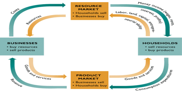
Source: Rookie Economics (n.d.).
The above mentioned diagram describes how business firms and households interact in the marketplace, namely in the input (‘resource market’) and the goods and services markets (‘product market’).
In the resource market, businesses have to incur in economic costs in order to produce goods and services. These organisational inputs essentially comprise labor, capital, and land (typically the property of households), and are brought by business firms as organisation resources to their corresponding transformative business processes. These organisational resources have to be paid to households, who see these costs as a form of payment for their supply of the said organisational resources, taking into consideration the prices associated to each of these factors of production in the resources market. In view of the fact that business firms are profit optimising firms, the goods and services produced by these firms will be sold at a profit in the product markets.
In the product markets, and once the transformative business leads to the production of the underlying goods and services, business firms sell these wares to households[3], who consume them as personal consumption expenditures. These consumption expenditures have to be paid for, thus constituting a source of revenue for the corresponding business firms. In turn, households thus consume these goods and services in order to continue to furnish organisational resources in the resources markets, and so forth.
It should be pointed out that the above mentioned diagram constitutes a very simplified representation of economic reality, as, for example, the complex role of the financial system is not addressed, as the introduction of credit would excessively complicate the underlying economic analysis. Moreover, both the resources and product markets are always in equilibrium, as markets clear according to the previously presented aggregate demand and supply curves, notwithstanding the fact that, in practical terms, markets do not always clear as neatly as the diagram would suggest. Thus, breaks in the diagram might occur when there are disruptions in the financial markets, such as the global financial crisis of 2007 - 2008, which strongly curtailed aggregate demand through a severe negative wealth effect caused by a fall in real estate prices. In this case, households’ spending patterns were negatively curtailed, leading firms to review their spending on the resources markets, which further negatively impacted households (their share of income accruing from the sale of business organisational inputs), and so forth.
8. Conclusion
In the context of a post-crisis environment, macroeconomic issues have been at the forefront of global economic debate. The present essay presents and describes some of the most essential macroeconomic concepts required to critically analyse contemporary global macroeconomic topics and issues of the utmost importance, using a range of simple, but effective economic models.
REFERENCES
Balderston, T., n.d. German hyperinflation. [Online]. Available: https://link.springer.com/chapter/10.1057%2F9780230280854_11 [viewed 2 August 2017].
Bank of England, 2017. Monetary Policy Framework. [Online]. Bank of England. [viewed 2 August 2017]. Available from: http://www.bankofengland.co.uk/monetarypolicy/Pages/framework/framework.aspx
Blanchard, O., 2009. Lessons of the Global Crisis for Macroeconomic Policy. [Online]. Available: https://www.imf.org/external/np/pp/eng/2009/021909.pdf [viewed 2 August 2017].
Economic Concepts, n.d. Determinants of National Income or Factors Affecting the National Income. [Online]. Available: http://economicsconcepts.com/determinants_of_national_income.htm [viewed 2 August 2017].
Economics Student Association, n.d. Welcome to the Economics Association. [Online]. Economics Student Association. [viewed 2 August 2017]. Available from: http://uec.syr.edu/
Krugman, P., Wells, R., and Grady, K., 2011. Essentials of Economics. Second edition. United States of America: Worth Publishers.
Lipsey, R., and Chrystal, A., 2015. Economics. 13th edition. United Kingdom: Oxford University Press.
Mishkin, F.S., 2015. The Economics of Money, Banking and Financial Markets. Eleventh global edition. United States of America: Pearson Education.
Rookie Economics, n.d. Circular Flow Model. [Online]. Rookie Economics. [viewed 2 August 2017]. Available from: https://stevenduan.wordpress.com/the-idea-of-economics/circular-flow-model/
Sloman, J., Wride, A., and Garratt, D., 2012. Economics. Eight edition. England: Pearson Education Limited.
Summers, P.M., 2005. What Caused The Great Moderation? Some Cross-Country Evidence. [Online]. Available: https://www.kansascityfed.org/publicat/econrev/pdf/3q05summ.pdf [viewed 2 August 2017].
Yellen, J.L., n.d. Aggregate Demand and the Global Economic Recovery. [Online]. Available: http://www.frbsf.org/economic-research/files/Yellen.pdf [viewed 2 August 2017].
[1] The goods and services might also be exported to other external markets. This case will be addressed when presenting the economic concept of Gross Domestic Product (G.D.P.).
[2] Price stability has historically been a source of great concern to central banks, although since the onset of the Great Moderation, global inflationary pressures have subsided, when compared to the historical inflation rates attained in the 1970’s and early 80’s (Summers, 2005).
[3] These goods and services might also be sold to other business firms and to the government, but, for the sake of simplicity, the latter two entities are generically treated as ‘households’, in order not to add excessive complexity to Figure 7.
Cite This Module
To export a reference to this article please select a referencing style below: